Artmis AI
Analyzing Revolutionary Trading Machines Independent Source


April 6, 2023
For E as a Mother , H as a Grandfather, M as a Shahmir
Release 0.10.1
"In God we trust, others must bring Data"
W. Edward Deming
ARTMIS ARTIFICIAL INTELLIGENCE is under the MIT License.
Introduction
This paper presents a solution using LSTM's deep neural network architecture, and the use of Keras and TensorFlow, to provide multidimensional time series forecasts in determining the stock value of global financial markets. Believe it or not, this program, which is artificial intelligence, has been able to accurately predict a stock market icon (with more than 98 percent accuracy) for the next 24 hours. I named the program based on this article ARTMIS AI for some reason.
Currently, ARTMIS has been able to achieve success in the pre-pin test of the live price of active valuation charts in all stock markets - (tested from S&P500 stocks in full and point in other markets) in the period of one second to 3 minutes with 99.23%, in the range of one second to 12 minutes with 99.79%, the period from one second to one hour with 99.04 The percentage and timeframe of one hour to one day, with 98.88% success, has been able to predict the data. To get the full results and log the program file via Github, proceed.
ARTMIS ability, especially in stock market data sets Features and graphs of the valuation of encrypted currencies, is because the input data is uninterrupted and does not require a re-analysis to provide stock price momentum indicators.
The current source code and ARTMIS framework are available in the GitHub fork but are not publicly available due to a lack of valuation. Therefore, it is necessary to access the source of ARTMIS through a pool request.
ARTMIS has now been upgraded to version 0.197.6. Through Python version 3.5, you can adapt the required programs and source code versions through the requirements.txt file. Note that deviations from these versions may cause errors in the performance of the program or the performance of ARTMIS.
However, the following article briefly addresses the neurons used in the LSTM-type ARTMIS, I will provide a very simple example of sinusoidal wave prediction, and then select a random timeframe through the components of the ARTMIS and run the program. Again, this article will introduce basic knowledge of deep neural networks as simple networks so that the concepts are fully conveyed.
Introduction to Stock Market Analysis
Stock market analysis is a process that involves the study of financial markets, such as stocks and bonds. It's important because it helps investors make better decisions when investing in stocks. The benefits of stock market analysis are many.
The ability to predict future trends based on historical data.
Understanding how different factors affect the value of a company's stock.
Identifying which sectors are performing well or poorly at any given time
Fundamental Analysis
Fundamental analysis is the study of economic factors that influence a company's share price. There are many different types of fundamental analysis, but they all involve examining a company's financial statements and other information to determine its value.
Fundamental analysts look at things like revenue growth rates, profit margins and debt levels when making investment decisions. They also consider whether there are any threats to the company's business model or industry position (such as competition from new entrants).
Technical Analysis
Technical analysis is a method of evaluating securities that focuses on price and volume data. It attempts to identify patterns in market activity, such as price trends, by analyzing statistical relationships between historical data. Technical analysts believe that future prices are determined by past prices and other factors (such as interest rates). They also believe that these trends can be discerned from historical data; therefore, they use charts or other tools to identify them.
Technical analysts make investment decisions based on these patterns rather than fundamental information about the company or industry being analyzed. For example, instead of looking at whether a company has strong growth prospects for its products or services--which would be considered "fundamental" analysis--a technical analyst might look at how quickly its share price has risen over time relative to other companies' shares in order determine whether it's a good investment opportunity now (assuming this has happened before).
What are LSTM neurons?
One of the major problems that plagued the architects of common neural networks for a long time was the impossibility of interpreting the sequence of inputs, which relied on each other to receive and process information and a platform fabrication. This information can be tandem words in a sentence, to allow a running platform to predict the next word, or it could be points of passing time that provides context based on undated events in that sequence.
In simple terms, neural networks are introduced, and with each run, they get an independent data vector.
I don't know how to investigate why no one has ever sought to answer this, but the main problem is that neural networks can't understand the concept of memory to use in tasks that require memory.
If we look at the concept of intelligence, we realize that intelligence, both for living organisms and machines, has the same meaning: the ability to model the changes surrounding that neural network, relative to the input and output data of that neural network in the same direction (time), human beings are not intelligent from birth, a human baby cannot survive alone, but over time, by observing the changes that have occurred around him. It falls, stores patterns in its memory and learns to walk and talk intelligently by knowing its behavior over the same time and creating a pattern of proportionality between the two.
Therefore, to predict the behavior of other variables in a subject at which time is similar to the neural network of the machine, a simple feedback-type approach for neurons should be used in the network.
In current neural networks, the output is given feedback to the input to provide the context in the last entries seen. These recursive neural networks (RNN) are called. While these RNNs work to some extent, they have a relatively big problem when using them over time. This is what they know as the gradient problem. Due to the lack of understanding of the concept of memory from the input and output of the network and adapting it to concurrent data, an effective environment arises.
For several reasons in this article, I prefer to say that RNNs are not suitable for solving many real-world problems due to the gradient problem.
This is where the Short-Term Memory Neural Network (LSTM) came to its aid. Like RNN neurons, LSTM neurons hold a background of memory in their pipeline to allow for the handling of sequential and temporal adaptable issues without affecting the gradient on their performance.
Many articles can be found online discussing the function of LSTM cells in great mathematical detail. However, in this article, I will not discuss the complex and extraordinary performance of LSTM, as I intend to explain ARTMIS and its performance.
To further understand the topic, come below a diagram of the typical inner function of an LSTM neuron. This includes several layers and point operations that act as a gateway to data input and output, and forgets to feed LSTM cell status. This cellular state is what maintains long-term memory and context across networks and inputs.
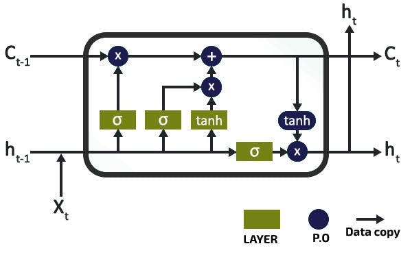
To demonstrate the use of LSTM neural networks in predicting time series, it is best to start with the most fundamental issue we can think about, i.e. A Sure Time Series: The Sinusoidal Wave. So I created the data that I need to model more of the fluctuations of this function to teach the LSTM network.
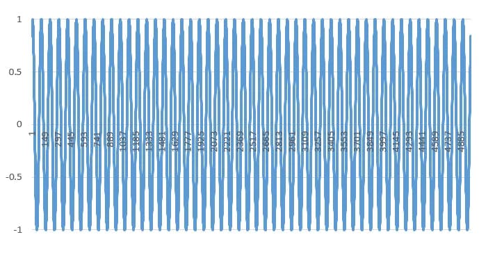
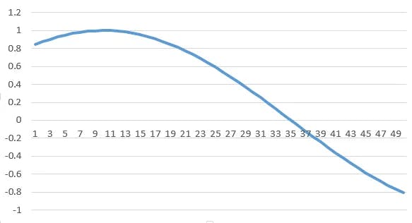
The data presented in the fork contains a file called sinewave.csv which includes 5,001 time periods of a sine wave, with an amplitude and frequency of one (and of course with an angular frequency of 6.28 degrees) and a time delta of one hundredth. The result of this is when drawing as follows:
So now that I have the data, I'm teaching the LMST to simply learn and feed the sine wave, through its proportionality to the size of the adjusted window of data, which I've given it.
LSTM is expected to be able to predict the next N-steps of the series and continue to output the sine wave.
Then we start by converting and loading data from the CSV file into a panda data frame, then used for output, a numpy array that feeds LSTM.
The Keras layers in LSTM work in this way by taking a disabling array of 3 dimensions (N, W, F) where N is, the number of instructional sequences, W is, the sequence length and F are the number of attributes of each sequence. Because of the current network constraints, I decided to use the sequence length (read window size) with the number fifty, which allows the network to process, so the LSTM of the sine waveform creates an image for itself and with this solution teaches itself to get the pattern of the sequences based on the previous window.
Sequences themselves are sliding windows. For this reason, each time a unit (time) is moved, they overlap with the previous windows. A typical learning window with a sequence length of fifty, when drawing on the grid, is shown below:
To load this data, I created a DataLoader class in my code to prepare a separate directory for the layer that loads the data.
Solution
You will notice that after initialization of an object in the DataLoader, the file name, along with a split variable, which determines the ratio of the information used to learn, versus the experimental patterning, and a column variable that allows selecting one or more columns of data, will be sent at the same time. For one-dimensional or multidimensional analysis ahead, the following code will come into force:
class DataLoader():


  def __init__(self, filename, split, cols):

    dataframe = pd.read_csv(filename)

    i_split = int(len(dataframe) * split)

    self.data_train = dataframe.get(cols).values[:i_split]

    self.data_test  = dataframe.get(cols).values[i_split:]

    self.len_train  = len(self.data_train)

    self.len_test   = len(self.data_test)

    self.len_train_windows = None


  def get_train_data(self, seq_len, normalise):

    data_x = []

    data_y = []

        for i in range(self.len_train - seq_len):

                  x, y = self._next_window(i, seq_len, normalise)

                  data_x.append(x)

                  data_y.append(y)

        return np.array(data_x), np.array(data_y)
After having a data object, which allows us to load data, I need to build a deep neural network model. Again, to hypothetically separate the framework, I create a code from a Model class next to the config.json file and teach the neural network to use it, to easily create an example of the model I created according to the required architecture and hyper met parameters stored in the configuration file.
So ()build_model is the main function that builds the network, and its functions take the parsed configuration file.
The function code can be seen below.
class  Model():

  def  __init__(self):
 self.model = Sequential()

  def  build_model(self, configs):
 timer = Timer()
 timer.start()

  for layer in configs['model']['layers']:
 neurons = layer['neurons'] if  'neurons'  in layer else  None
 dropout_rate = layer['rate'] if  'rate'  in layer else  None
 activation = layer['activation'] if  'activation'  in layer else  None
 return_seq = layer['return_seq'] if   'return_seq'  in layer else  None
 input_timesteps = layer['input_timesteps'] if  'input_timesteps'  in layer else  None
 input_dim = layer['input_dim'] if  'input_dim'  in layer else  None

  if layer[ 'type'] == 'dense':
 self.model.add(Dense(neurons, activation=activation))
  if layer['type'] == 'lstm':
 self.model.add(LSTM(neurons, input_shape=(input_timesteps, input_dim), return_sequences=return_seq))
  if layer['type'] == 'dropout':
 self.model.add(Dropout(dropout_rate))

 self.model. compile(loss=configs['model']['loss'], optimizer=configs['model']['optimizer'])

  print('[Model] Model Compiled')
 timer.stop()
By loading the built-in data and model, it is now possible to continue training the model with educational data. I created a separate implementation module that imagines the data output from the Model and DataLoader separation and their combination of neural network learning.
See below the general enforcement string code for neural network model training
configs = json.load(open('config.json', 'r'))


data = DataLoader(

    os.path.join('data', configs['data']['filename']),

    configs['data']['train_test_split'],

    configs['data']['columns']

)


model = Model()

model.build_model(configs)

x, y = data.get_train_data(

    seq_len = configs['data']['sequence_length'],

    normalise = configs['data']['normalise']

)


model.train(

    x,

    y,

    epochs = configs['training']['epochs'],

    batch_size = configs['training']['batch_size']

)


x_test, y_test = data.get_test_data(

    seq_len = configs['data']['sequence_length'],

    normalise = configs['data']['normalise']

)
Well, now for output, we run two types of predictions, then from the result we get, we execute the third prediction:
A. Point to Point Analysis
Which means I just predict one point at a time, and I draw this point as a prediction for the ARTMIS network, then I add the next window.
B. Sequence Analysis
So I'll initialize a training window with the first part of the training data just once. Then Artmis predicts the next dot model, and like the point-to-point method, I will change the window. The difference between the two is that using the data I had imagined in the previous forecast, I create a new prediction, which in the second step means that there will only be one data point (last point) than the previous forecast.
Forecast
Now in the third forecast, there will be the last two data points from the previous forecasts and (more) that after fifty predictions, the ARTMIS model practically predicts itself based on the previous forecasts it has achieved. This method finally allows us to use the whole model to predict future time steps,
Below you can see the code and outputs of the models for point-to-point predictions and full sequence predictions:
def predict_point_by_point(self, data):
    #Predict each timestep given the last sequence of true data, in effect only predicting 1 step ahead each time
    predicted = self.model.predict(data)
    predicted = np.reshape(predicted, (predicted.size,))
    return predicted

def predict_sequence_full(self, data, window_size):
    #Shift the window by 1 new prediction each time, re-run predictions on new window
    curr_frame = data[0]
    predicted = []
    for i in range(len(data)):
        predicted.append(self.model.predict(curr_frame[newaxis,:,:])[0,0])
        curr_frame = curr_frame[1:]
        curr_frame = np.insert(curr_frame, [window_size-2], predicted[-1], axis=0)
    return predicted

predictions_pointbypoint = model.predict_point_by_point(x_test)
plot_results(predictions_pointbypoint, y_test)

predictions_fullseq = model.predict_sequence_full(x_test, configs['data']['sequence_length'])
plot_results(predictions_fullseq, y_test)
{
    "data": {
        "filename": "sinewave.csv",
        "columns": [
            "sinewave"
        ],
        "sequence_length": 50,
        "train_test_split": 0.8,
        "normalise": false
    },
    "training": {
        "epochs": 2,
        "batch_size": 32
    },
    "model": {
        "loss": "mse",
        "optimizer": "adam",
        "layers": [
            {
                "type": "lstm",
                "neurons": 50,
                "input_timesteps": 49,
                "input_dim": 1,
                "return_seq": true
            },
            {
                "type": "dropout",
                "rate": 0.05
            },
            {
                "type": "lstm",
                "neurons": 100,
                "return_seq": false
            },
            {
                "type": "dropout",
                "rate": 0.05
            },
            {
                "type": "dense",
                "neurons": 1,
                "activation": "linear"
            }
        ]
    }
}
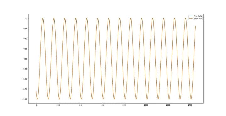
Now with real data coverage, I can see that with just 1 course and a small training set of data, the LSTM deep neural network has already done a very good job of predicting sinusoidal performance.
Sine prediction photo of half an hour number 19, but the point is that now more and more in the future time, the margin of error increases, because the errors of previous predictions become more and more, that as the windows reach the present time and the actual data matches the predictions of ARTMIS, I can use the initial function to compare the predicted error with the data. Real data that have reached the present time (and are available to ARTMIS ) and the adaptation of these data to the predictions made and the study of the tolerance pattern of real data and predictions, can easily be reduced to almost zero. Because this match first adapts from the initial prediction to the present error and searches for the patterning, secondly, with each opening of the new window, if the error rate is less than three-tenths of a percent, it considers the patterning as a successful prediction. This method causes ARTMIS to check for the correct prediction of the next second every second. So in the example of the full sequence, the more we predict in the future, the more accurate the tolerance and scope of the predictions are with the actual data.
But, we have to consider that since the sin function is a very easy oscillating function with zero noise, ARTMIS can predict it to a good extent without overprocessing, this is very important because it is possible to easily fit the model by increasing periods and removing excessive drop layers to create it. Therefore, in the test implementation of the sinusoidal function without noise and without overprocessing the data, the prediction of ARTMIS is quite accurate, which is of course the experimental data pattern that has been successful.
Real Data
Next, let's use the models that are going live in real-world data to see the effects.
So far, ARTMIS has predicted more than 700 temporal functions of a sine wave based on the exact point-to-point basis. So, now I have to do the same in a stock market time series to check out ARTMIS'ES prediction model in the real world.
I used the charts on the site capital.com, got an API from site to head and selected DOT/USD, US500/USD and BTC/USD charts to run.
The problem is that, unlike the sine wave, the time series of the stock market is not at all a specific constant function from which to extract a specific pattern, so I can't draw it. But the solution I found is that the best feature to describe the movement of the time series of a stock market chart is the implementation of the chart randomly.
That is, as a random process, a real random implementation has no predictable pattern and therefore it would be pointless to try to model it. But it's surprising that fortunately, from many of the fanatics in these markets, there are persistent arguments that the stock market is not a completely random process (I heard this from one of the market participants a month ago), so this claim led me to assume that the time series of stock market charts might have some kind of hidden pattern that could not be understood by the human mind, in fact finding these patterns. It was hidden which made me use deep LSTM networks as neural networks.
The data I used to run this test is in the us500.csv file in the Data folder on the GitHub site. This file includes open prices, high, low, and closed prices as well as the daily volume of the US500 stock index from January 2010 to September 2022.
One Dimensional Model
Firstly, I just created a one-dimensional model using just the closing price. By matching the config.json file to reflect live data, I kept most parameters constant, only one change that needs to be made is that unlike the sine wave, which only had a numerical range between -1 and +1, the price of these shares is an absolute price that is constantly changing in the stock market. That is, if I tried to teach ARTMIS without vectors and normalization, the result would never have converged.
To combat this, which spreads like iron rust to all the components of the ARTMIS, I separate each n-sized window from the previous data and predictions and normalize its information based on the outcome of the data change to get the percentage of data changes from the beginning of that window to the present. So the data at point i=0 will always be 0.
I used the following equations to normalize (at first) and eccentricity (at the end of the prediction process) so that a number from the real world could be out of the forecast:
I added the normalise_windows() function to my DataLoader class to perform this conversion, I will create a normalization flag (with a dollar symbol) in the configuration file to identify the actual vector information, which indicates the normalization of these windows.
def normalise_windows(self, window_data, single_window=False):
    '''Normalise window with a base value of zero'''
    normalised_data = []
    window_data = [window_data] if single_window else window_data
    for window in window_data:
        normalised_window = []
        for col_i in range(window.shape[1]):
            normalised_col = [((float(p) / float(window[0, col_i])) - 1) for p in window[:, col_i]]
            normalised_window.append(normalised_col)
                # reshape and transpose array back into original multidimensional format
        normalised_window = np.array(normalised_window).T
        normalised_data.append(normalised_window)
    return np.array(normalised_data)
As Windows normalizes, I can now run the model the same way it did with sine wave data. But we have to note that, we made a very important change when running this data. That is, instead of using the model train method that exists within the ARTMIS framework, we use the model.train_generator() and we normalize ourselves as real data. why are we doing this?
In the first experimental implementation of this method with real data, I realized that when I was teaching real big data to ARTMIS AI, as soon as the result started, the temporary memory easily erased itself. Because of the model. train function () is forced to first load all the complete real data into the machine's temporary memory, then to run the vector and normalize the actual data, it is necessary to regain access to each time window and execute the resulting changes on them, causing the memory overflow to be applied in the memory emptying command.
So, instead of using this command, I used Keras's fit_generator function to allow ARTMIS to dynamically learn real datasets using a Python generator to draw data, which means memory usage is dramatically minimized.
configs = json.load(open('config.json', 'r'))

data = DataLoader(
    os.path.join('data', configs['data']['filename']),
    configs['data']['train_test_split'],
    configs['data']['columns']
)

model = Model()
model.build_model(configs)
x, y = data.get_train_data(
    seq_len = configs['data']['sequence_length'],
    normalise = configs['data']['normalise']
)

# out-of memory generative training
steps_per_epoch = math.ceil((data.len_train - configs['data']['sequence_length']) / configs['training']['batch_size'])
model.train_generator(
    data_gen = data.generate_train_batch(
        seq_len = configs['data']['sequence_length'],
        batch_size = configs['training']['batch_size'],
        normalise = configs['data']['normalise']
    ),
    epochs = configs['training']['epochs'],
    batch_size = configs['training']['batch_size'],
    steps_per_epoch = steps_per_epoch
)

x_test, y_test = data.get_test_data(
    seq_len = configs['data']['sequence_length'],
    normalise = configs['data']['normalise']
)

predictions_multiseq = model.predict_sequences_multiple(x_test, configs['data']['sequence_length'], configs['data']['sequence_length'])
predictions_fullseq = model.predict_sequence_full(x_test, configs['data']['sequence_length'])
predictions_pointbypoint = model.predict_point_by_point(x_test)

plot_results_multiple(predictions_multiseq, y_test, configs['data']['sequence_length'])
plot_results(predictions_fullseq, y_test)
plot_results(predictions_pointbypoint, y_test)
{
    "data": {
        "filename": "sp500.csv",
        "columns": [
            "Close"
        ],
        "sequence_length": 50,
        "train_test_split": 0.85,
        "normalise": true
    },
    "training": {
        "epochs": 1,
        "batch_size": 32
    },
    "model": {
        "loss": "mse",
        "optimizer": "adam",
        "layers": [
            {
                "type": "lstm",
                "neurons": 100,
                "input_timesteps": 49,
                "input_dim": 1,
                "return_seq": true
            },
            {
                "type": "dropout",
                "rate": 0.2
            },
            {
                "type": "lstm",
                "neurons": 100,
                "return_seq": true
            },
            {
                "type": "lstm",
                "neurons": 100,
                "return_seq": false
            },
            {
                "type": "dropout",
                "rate": 0.2
            },
            {
                "type": "dense",
                "neurons": 1,
                "activation": "linear"
            }
        ]
    }
}
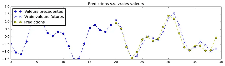
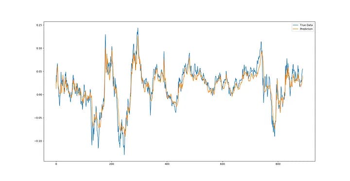
The execution of real resulted in from and re-realized data, in a point-to-point forecast, as stated above, in the output predicted information that fits perfectly with reality. It's both a matter of joy and concern because its simplicity is a bit glamorous!
So more closely, I noticed that the predicted data line is composed of separate prediction points that have passed its entire previous actual windows! Because I defined the movement of the timeline as constant and unstoppable, ARTMIS no longer needs to look at and understand a lot of things about the timeline itself, as if he understood that he had to move along the timeline. And he has taught himself that in his movement in the vector of time, he is far from the next point of a unit, and can draw his movement by taking into account the prediction of the next point, up to n points after that as the visualization of the previous points. This means that ARTMIS understands and learns the present, the past and the future over what he is doing. Therefore, even if he has made a mistake in predicting a point in the present time, he can correct them by factoring in his next predictions and making a more accurate pattern by ignoring his mistake and changing the wrong prediction with real information.
This means that ARTMIS is reviewing the prediction process at the time of execution, in case the actual data mismatches with the data he has obtained in the present, corrects his future predictions (which he processes within the neural network) and ignores his wrong prediction, thus reconfirming the prediction with the actual information he has in his memory from the past. future and continues to work, and because you ignore your error and replace it, it again allows itself to make an error, which is always a window number.
Although this may not seem promising in the early stages of its learning due to the start of ARTMIS's work, for accurate forecasting of the next price (since the forecasts are first as non-decimal ranges and have fewer resources to match the forecast and real prices), it will become more accurate every second of its implementation and even at this moment has important applications. While it now doesn't know how much the next exact price will be, it offers a very detailed representation of the range of where the next price should be.
This information can be used in applications such as forecasting volatility (apparently the cyclical predictability of high or low volatility in the market can be very beneficial for a high-investment trading strategy) or getting out of a trade can be used as a precise indicator. ARTMIS can obtain anomaly detection just by predicting the next point, then comparing it to actual data on arrival, and if the actual data value differs significantly from the predicted point, the anomaly flag can be passed for that point of the token data.
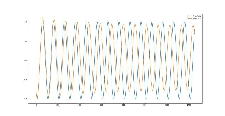
Moving towards full sequence prediction, ARTMIS seems to have predicted the least usefulness for these types of time series – he learned this model by himself with over parameters – we can see a slight bulge at the start of the forecast where real prices somehow follow the continuity movement. However, ARTMIS decides very quickly. The most optimal pattern for prediction is convergence to some time series equilibrium. So far, it has been able to accurately predict the price return.
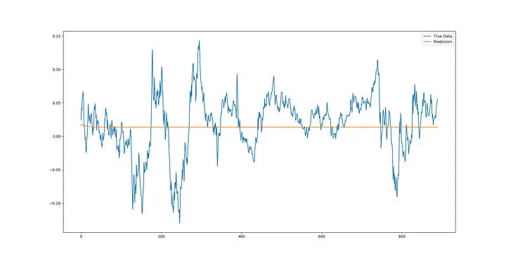
I ran ARTMIS for real market forecasting, which I call SRG PREDICTION (in honor of Paul Seaverson, Michael Reid and David Goldschleg, creators of DarkWeb). The combination of full sequence prediction and matching of previous data is real and means continuously comparing the new time window with the initial test data, predicting the next point and creating a new window with the next point and going further in time. However, when it reaches the point where the input window is completely composed of past forecasts, Stops the execution of the prediction process in that window, compares the actual data to the forecast, ignores the error, executes a new pattern factor by matching the error and predicting the windows after that, re-comparing it to the actual data in the previous windows, and at the same time continues to execute the forecast, and a full window length moves forward, then Resets the new window with actual test data and continues the forecasting process. In essence, these predictions run a different trend line on the previous data so that it can analyze and make the prediction data more accurate.
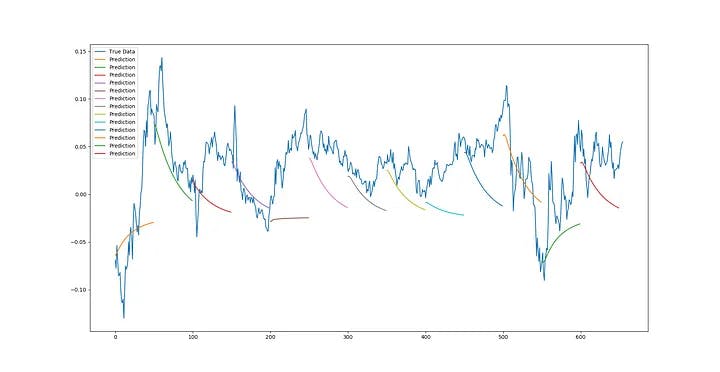
We can see from multiple sequence forecasts that ARTMIS seems to correctly predict trends (and trend ranges) for most time series. Undoubtedly, it is possible to achieve more accuracy by fine-tuning the ultraparametrics.
the forecast has only received one-dimensional inputs so far (the "closing" price on the S&P500 dataset). That's because my machines are unable to simultaneously execute ARTMIS predictions due to other programs, but with more complex data sets, there are naturally different dimensions to the sequences that can be used to improve the dataset, thereby increasing the accuracy of the ARTMIS.
In the case of the S&P500 dataset, one can teach ARTMIS to get Open, High, Low, Close and Volume, forming five possible dimensions. ARTMIS can use multidimensional input datasets with the program I wrote for, so all you have to do to use ARTMIS is to change the columns and values of the input_dim the first layer of lstm appropriately to implement the multidimensional model. So in this case, I run the ARTMIS model using two dimensions: "close" and "volume".
{
    "data": {
        "filename": "sp500.csv",
        "columns": [
            "Close",
            "Volume"
        ],
        "sequence_length": 50,
        "train_test_split": 0.85,
        "normalise": true
    },
    "training": {
        "epochs": 1,
        "batch_size": 32
    },
    "model": {
        "loss": "mse",
        "optimizer": "adam",
        "layers": [
            {
                "type": "lstm",
                "neurons": 100,
                "input_timesteps": 49,
                "input_dim": 2,
                "return_seq": true
            },
            {
                "type": "dropout",
                "rate": 0.2
            },
            {
                "type": "lstm",
                "neurons": 100,
                "return_seq": true
            },
            {
                "type": "lstm",
                "neurons": 100,
                "return_seq": false
            },
            {
                "type": "dropout",
                "rate": 0.2
            },
            {
                "type": "dense",
                "neurons": 1,
                "activation": "linear"
            }
        ]
    }
}
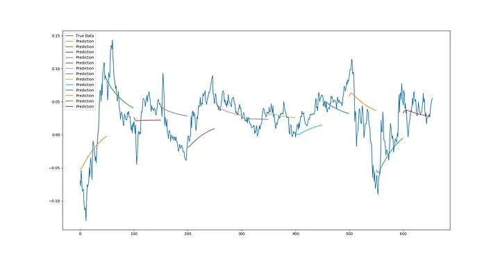
With the addition of the second dimension of "Volume" next to "Close", it can be seen that the output forecast becomes much more accurate. Predictive trend lines seem to be more accurate for predicting future minor downpours, not only the prevailing trend from the beginning but also the accuracy of trend lines to improve in this particular case.
while the purpose of this paper is to provide a functional example of the deep LSTM neural networks in the Sereno program, only the level of potential and application of them in consecutive and temporal problems I specified.
At the time of writing this text, LSTMs have been successfully used in many real-world problems ranging from the classic time series issues described here, to automatic text correction, anomaly detection and fraud detection, to having nuclear in Tesla vehicle technologies.
Currently, LSTMs offer significant improvements in more classical statistical time series approaches in modeling nonlinear relationships and the ability to process data with multiple dimensions by a non-linear method.
The full source code of the written ARTMIS platform can be viewed under a GNU General Public License (GPLv3) on my GitHub page. I just request that you do not change the validity of its construction, which is under the name ***** on the page******* .
Update :
Here I present the process of learning ARTMIS first based on the sine wave and then based on real waves. The issue that should be noted is that the explanations provided in this article are written briefly and for several reasons for the simplicity of the subject for the reader. Unfortunately, due to copyright issues, I did not publish the source code of this program, which I hope can be made available to the public shortly.
The next thing is that many people (including myself until a while ago) believe that there is no particular pattern in the movement of stock market symbols and can never predict the trend of movement. But at the time of ARTMIS's experiment and learning, I noticed that in some time intervals, there was suddenly a sharp difference in the slope of the forecast chart, with the actual chart, which is quite strange, because ARTMIS's performance is such that when the actual data matches the forecasts in the present time, ARTMIS checks every window that is created. Be, check it and ignore the error in case of a prediction error. Therefore, creating a slope of difference requiring at least 3 50-unit windows does not make sense in ARTMIS's performance.
After analyzing the windows, I noticed that because of the change in real market prices, in loading the chart, such a slope is created, because the windows intended for ARTMIS are defined in a second range, and the change in the angle of the stock market charts is five seconds. This gradient change is logical and by changing the error of ARTMIS instead of every second, the problem was resolved every 5 seconds.
But it made me think that to be more accurate, we can create data from global news and its impact on stock values that help you learn Serena and forecasts.
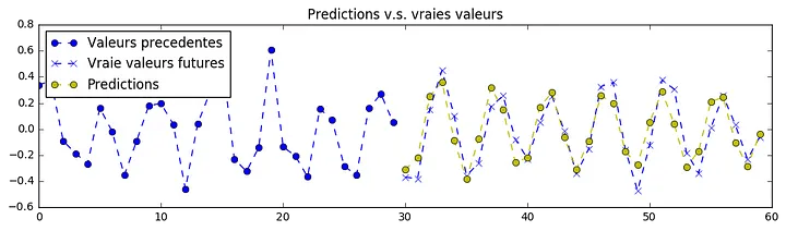
So after studying a lot of articles about the impact of news on the value of global stocks, I realized that it's not the news itself that affects valuations, but the reaction of people to that news that has a strong impact on stock values, so by creating a database of searching for certain words that are searched every minute by people on Google, I was able to bring the sentiment involved in the market to ARTMIS . I teach. In this way, new data was added to the dimensions of ARTMIS input data. I'll show you the results from the sine wave as diagram below. The yellow line is ARTMIS's prediction.
Update
With the addition of a new dimension to the input data of so-called market sentiment analysis using another algorithm and connecting it to the data input as a layer of the small neural network, I released a new version of ARTMIS. So now ARTMIS has been upgraded to version 1.199.6. Read more here.